Training without Data - PINNs¤
![]()
This example demonstrates one possible way of training a physics-informed neural network (PINN)-style model without any data using klax.fit. Alongside, we demonstrate how to define user-defined custom loss function based on the klax.Loss protocol and how implement and log custom training klax.Metrics.
To run it locally install klax with plotting capability via pip install 'klax[plot]'.
We start by importing the required packages for model creation, optimization and plotting.
import equinox as eqx
import jax
import jax.numpy as jnp
import jax.random as jr
import optax
from jaxtyping import Array, PRNGKeyArray
from matplotlib import pyplot as plt

import klax
Here we want to find the solution \(u:\mathbb{R}\rightarrow\mathbb{R}\) of the ODE: $$ \begin{equation} \frac{\partial u}{\partial x} + u = 0, \quad u(x=0)=1 \end{equation} $$
The following code cell implements a PINN model as an Equinox module. It uses a small klax.nn.MLP to represent the solution field \(u(x)\). The model is trained by minimizing the residual of the ODE and the boundary condition on a set of collocation points \(x_i\), which are stored in the attribute x_collocation. The residual loss function itself is implemented as a static method model and decorated as a klax.Loss, making it compatible with klax.fit.
Note
Fore more complex PINN training, writing a custom fit method with random sampling of collocation points, gradient-based loss balancing and other optimization methods may be preferred. For more information see e.g. Wang et al. (2023) "An Expert's Guide to Training Physics-informed Neural Network". Meanwhile, the goal of this example is simply to show how training without data could be implemented using klax.
class PINN(eqx.Module):
    """A simple PINN-style model that solves the ODE u_x + u = 0 with u(0) = 1."""

    mlp: klax.nn.MLP
    x_collocation: Array  # Residual evaluation points

    def __init__(self, x_collocation: Array, key: PRNGKeyArray):
        self.x_collocation = x_collocation
        self.mlp = klax.nn.MLP(
            "scalar", "scalar", 2 * [16], activation=jax.nn.softplus, key=key
        )

    def __call__(self, x):
        return self.mlp(x)

    @klax.loss  # This method is a klax.Loss object
    @staticmethod
    def residual_loss(model, batch, run_state):
        """ODE residual and boundary condition redidual loss.

        We define a loss function that penalizes the residual of the ODE
        u_x + u = 0 and violations of the boundary conditions u(0) = 1.

        """
        ode_loss = model.ode_loss(model)
        bc_loss = model.bc_loss(model)
        return ode_loss + 0.1 * bc_loss  # Manual loss balancing

    @staticmethod
    def ode_loss(model):
        # Manually exclude x_collocation from optimization
        x_collocation = jax.lax.stop_gradient(model.x_collocation)

        # ODE residual
        u, u_x = jax.vmap(jax.value_and_grad(model))(x_collocation)
        residual = u_x + u
        return jnp.mean(residual**2)

    @staticmethod
    def bc_loss(model):
        # Boundary conditions
        bc_0 = model(jnp.array(0.0)) - 1.0
        return bc_0**2
Before training the model, let's define some custom metric such that we can track the ODE redisual and boundary condition losses independently during training. We set the vebosity to True such that the values will also be displayed in the training progress bar.
@klax.metric(name="bc_residual", verbose=True)
def bc_loss_metric(ctx: klax.TrainingContext):
    model = ctx.state.model
    return model.bc_loss(model)


@klax.metric(name="ode_residual", verbose=True)
def ode_loss_metric(ctx: klax.TrainingContext):
    model = ctx.state.model
    return model.ode_loss(model)
Lets train the model. First we provide the residual evaluation points x_collocation to initialize the PINN model. Here we choose \(x_i \in [0,1]\). Then we fit the model using the klax.fit method. Here, we pass residual to the loss argument as well as a list of klax.Metrics.
Note that we use data=None, since the model is trained without any labeled data (except for the Dirichlet boundary conditions) and the residual evaluation points are stored within the model itself. Importantly, we also have to specify that our data does not have any batch_axes.
x_collocation = jnp.linspace(0, 1, 100)
model_key, training_key = jr.split(jr.key(0))
model = PINN(x_collocation, key=model_key)
model, history = klax.fit(
model,
data=None,
batch_axes=None,
steps=100_000,
optimizer=optax.adam(1e-5),
loss=model.residual_loss,
metrics=(ode_loss_metric, bc_loss_metric),
key=training_key,
)
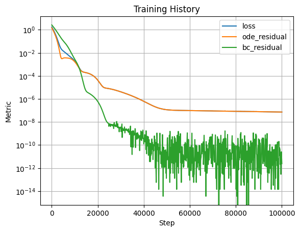
history.plot()
plt.show()
0%| | 0/100000 [00:00<?, ?it/s]
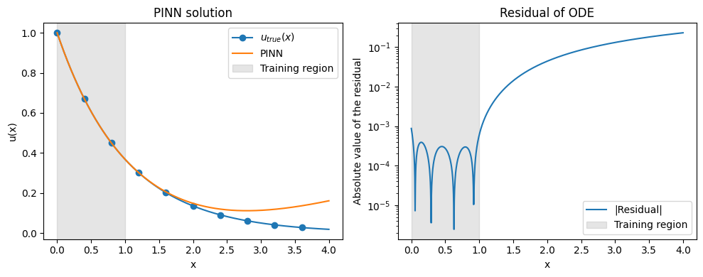
Finally, lets have a look at the model performance on the interval \([0,4]\) and compare it to the analytical solution \(u(x)=e^{-x}\).
def solution(x):
    """Compute the true solution of the ODE u_x + u = 0 with u(0) = 1."""
    return jnp.exp(-x)


def ode_residual(x):
    """Compute the ODE residual for a single collocation point."""
    u, u_x = jax.value_and_grad(model)(x)
    return u_x + u


x = jnp.linspace(0, 4, 1000)
u_true = jax.vmap(solution)(x)
u = jax.vmap(model)(x)
residual = jax.vmap(ode_residual)(x)

fig, axes = plt.subplots(1, 2, figsize=(10, 4))
axes[0].plot(x, u_true, marker="o", markevery=100, label=R"$u_{true}(x)$")
axes[0].plot(x, u, label="PINN")
axes[0].set(
    title="PINN solution",
    xlabel="x",
    ylabel="u(x)",
)
axes[0].axvspan(
    model.x_collocation.min(),
    model.x_collocation.max(),
    color="gray",
    alpha=0.2,
    label="Training region",
)
axes[0].legend()

axes[1].plot(x, jnp.abs(residual), label="|Residual|")
axes[1].set(
    title="Residual of ODE",
    xlabel="x",
    ylabel="Absolute value of the residual",
    yscale="log",
)
axes[1].axvspan(
    model.x_collocation.min(),
    model.x_collocation.max(),
    color="gray",
    alpha=0.2,
    label="Training region",
)
axes[1].legend()

plt.tight_layout()
plt.show()